Everyone's hyped about LLMs these days. It does amazing things—seems to think, looks smart, even intelligent. Naturally, I got curious: How does it "think"? How can it respond so well? And perhaps most intriguingly - Am I just a biological LLM? Do they process information anything like we do? Are there even some similarities?
Demystifying Neural Networks: Beyond Buzzwords. Part 1
2025-18-0218 min read
AIDeep LearningInteractive

Dots, Lines and Squiggles
The Tale of Gauss and the Lost Planet Ceres
Historical Context
In the early 1800s, long before influencers and viral tweets, astronomers were the celebrities. Navigating ships relied on stars, so discovering a new celestial body was a big deal. People even believed in magic and astrology—the positions of planets were thought to determine your fate. Today, while we like to think we've moved past such beliefs, many still cling to the "magic" of AI and ChatGPT prompts.
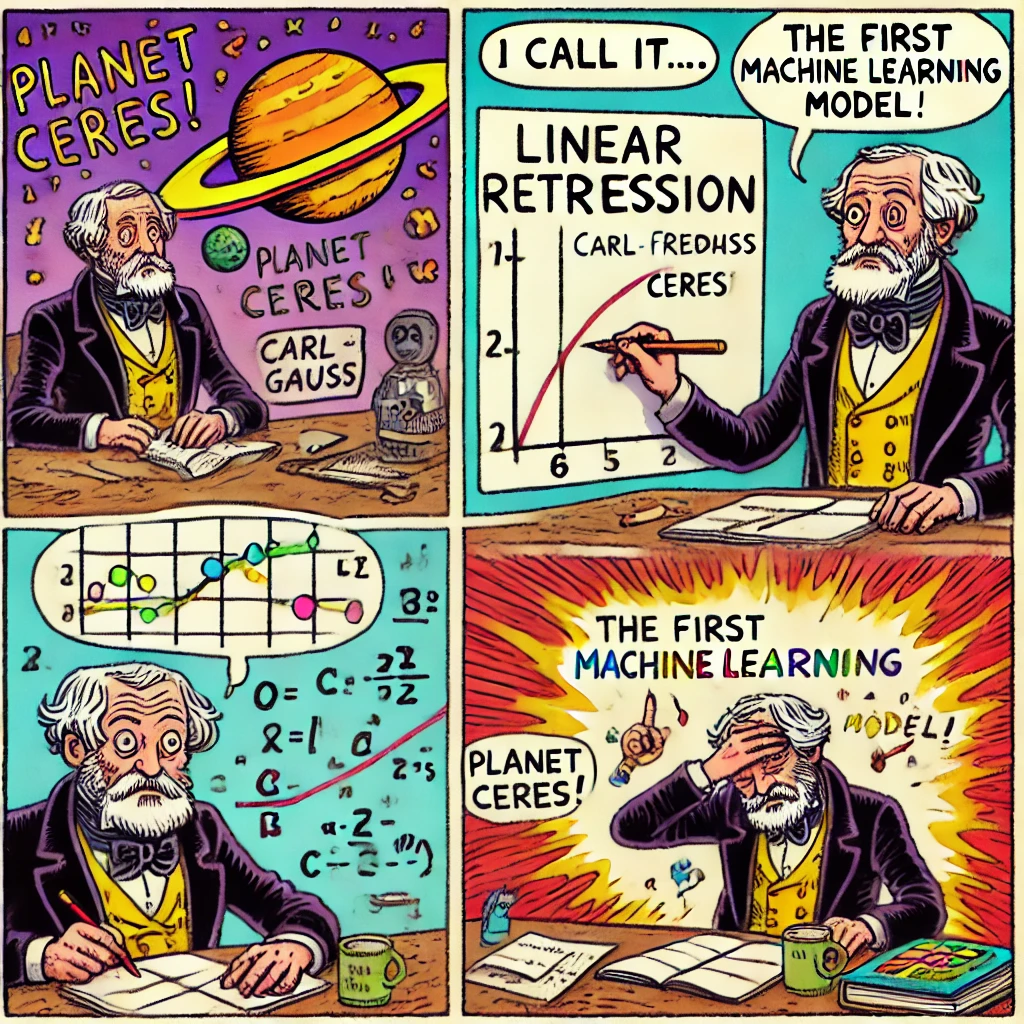
Our Machine Learning story begins on January 1, 1801, when Italian astronomer Giuseppe Piazzi spotted something new in the sky — he called it Ceres. Unsure if it was a comet or planet, he recorded its position 19 times over 42 days until it drifted too close to the Sun. The big question was: When and where would Ceres reappear? It became a race for the top astronomers of the time to predict its return.
Then there were this German guy Carl Friedrich Gauss. Using Piazzi's data and a form of machine learning (though with pen and paper(pen-and-paper learning) instead of silicon machines), he built a model of Ceres’s orbit. On December 7, 1801, Ceres reappeared just half a degree away from Gauss's prediction.
The Equation of a Line
Imagine plotting the positions of Ceres over time on a graph. On the x-axis, we have time—the days that Piazzi recorded Ceres. On the y-axis, we have position—simplified here as an angle to show where Ceres was in the sky.
When Gauss connected these points, they roughly formed a line. This gave him an idea: if the past positions line up in a predictable way, then maybe the next position will also be along that same line.
To understand how Gauss might have approached this problem, we need to know what makes a line a line. Every straight line in mathematics can be described by a simple relationship between two variables. For each step we take along the x-axis, we take a consistent step up or down on the y-axis. Mathematicians write this relationship as:
- m: The slope of the line, indicating how fast Ceres's position changes over time. A steeper slope means Ceres is moving faster.
- b: The y-intercept – the starting point on the y-axis, showing where Ceres was first observed.
- x: Your input value (in Gauss's case, the time).
- y: The predicted output (Ceres's position).
Try adjusting the slope (m) and y-intercept (b). Can you make the line fit the points better?
💡 Hint: The slope controls how steep the line is, while the y-intercept moves the entire line up or down.
Which Line Fits Best?
But there are multiple—actually, an infinite number of—lines we could draw that come close to our data points. How do we decide which one is the best fit? Should we just eyeball it and pick the one that looks closest? That might work for a human, but what we really want is for a machine to do this for us.
To do that, we need a way to compare lines objectively. We need a scoring system that tells us, with numbers, how well each line fits the data.
Mean Squared Error (MSE)
One way to score how well a line fits our data is by using something called Mean Squared Error (MSE). Think of MSE as a way to give each line a score, telling us how close it is to all the data points.
Here's how it works:
- Calculate the Error for Each Point: For each point on the graph, measure how far away the point is from the line. This difference is called the error—it tells us how much our prediction (the line) is off from the actual data point.
- Square Each Error: We then square these errors. Squaring serves two purposes:
- It makes all the values positive so that no errors cancel each other out.
- It also amplifies larger errors, making them more significant, which helps us focus on the big mistakes.
- Find the Average: Finally, we average all these squared errors. This average is called the Mean Squared Error (MSE). The smaller the MSE, the better our line fits the data points.
A low MSE means the line is really close to all the data points, while a high MSE means the line is far off. The goal? Minimize the MSE to find the best-fitting line.
By using MSE, we give each line a clear, numerical score—making it easy to compare different lines and pick the one that does the best job of predicting the data.
The formula for Mean Squared Error (MSE) is:
In this formula, is calculated from our line equation:. For each data point, we plug in the corresponding x-value to get .
The difference between Y_measured (the actual value) and Y_predicted gives us the error for that point. Squaring these errors helps us quantify how well our line fits the entire dataset.
👉 Adjust the line below and see how the MSE changes in real-time!
Ypred 1 = mx + b = (2.00)(1) + (-1.00)
Ypred 1 = 1.00
(Ymeasured 1 - Ypred 1)² = (0.50 - 1.00)² =0.2500
67.4100
MSE:8.4262
And? Where's the learning? Where's the Machine?
So far, we've been adjusting the line manually—tweaking parameters and eyeballing the best fit. But isn't machine learning supposed to learn without all this manual effort? What does it mean to "learn"? Gauss, back in 1801, was following a methodical procedure—adjusting his calculations to find the best fit for the observed data points. Learning, in this context, is about finding patterns or rules that best describe or predict data. He wasn't blindly guessing; he refined his predictions based on how well they matched reality. Without silicon or wires, Gauss was essentially performing a form of "manual machine learning," iterating toward the best explanation of Ceres's motion. Today, we let computers do the same—but faster, at scale. The basic idea remains the same; the difference is that now, silicon automates what once took weeks of calculations by hand. Let's dig deeper and see how this idea of learning translates into modern algorithms.
The Power of Derivatives: Finding the Best Fit Automatically
Now that we have a way to score how well a line fits the data using MSE, the next question is: how do we find the best possible line automatically?
What is a Derivative & Why Do We Need It? A Simple Guide
A derivative measures how something changes —it's essentially the rate of change (, means how fast y changes with respect to x). Imagine watching how something changes—like the steepness of a hill. A derivative tells you exactly how steep the curve is at a given point. When we talk about a line, the derivative gives us the slope—the rate of change of y with respect to x. It answers questions like: Is the line getting steeper or more flat? Is it increasing or decreasing?
However, remember that our error function depends on two parameters: the slope () and the intercept (). This means that rather than relying on a single derivative, we must consider two partial derivatives. The first, , measures how the error changes when only the slope is adjusted. The second, , reveals how the error shifts when the intercept is tweaked. Taking both into account provides a complete picture of the error landscape and sets the stage for effective optimization.
The Derivative of MSE
First, we focus on our line equation:
Our goal is to adjust the slope () to get the best possible fit. But to do this, we need to understand: how does changing affect the overall error? This is where the derivative comes in. The derivative helps us understand how changing m affects the overall error. For now, we'll keep fixed and see what happens as we adjust
The derivative value tells us two crucial things for each parameter:
- Direction: Which way to adjust the parameter to reduce error
- Magnitude: How strongly we should adjust it based on current mismatch
The partial derivatives for slope is:
Where α is the learning rate. Notice how each parameter update uses the current value of the other parameter - this interdependence is why we must update them together.
This tells us exactly how to adjust the slope to make the line fit better!
Watch how the error changes as you adjust the slope:
In our earlier exploration, we simplified the problem by keeping the intercept fixed so that we could clearly observe the impact of adjusting the slope on the Mean Squared Error. However, for our particular example we are taking two derivatives—one with respect to and one with respect to —to capture the full interdependent behavior of the error function. Try to adjust both the slope and intercept to see the error plot change.
Slope (m)
Intercept (b)
A Practical Challenge: Why Not Just Solve for the Derivatives Directly?
Imagine you're trying to find the bottom of a very hilly, rugged landscape. In calculus, the "gradient" tells you which way the land slopes downward at any point—like the steepness of a hill. For a simple, smooth hill, you might be able to work out exactly where the slope becomes zero (that is, where you're at the very bottom) by solving an equation. This is what we mean by "setting to find the minimum error.
However, in most machine learning problems the "landscape" (or error surface) is extremely complicated and has millions of dimensions. Here's why solving the equations directly isn't practical:
Interdependent Parameters
In a simple case, like fitting a straight line () to data, the errors depend on both (the slope) and (the intercept). Changing can affect the best value for and vice versa. In deep learning models, with millions of parameters, each parameter's effect is intertwined with many others. Solving one equation without considering the others simply isn't possible.
Complex and Rugged Error Surface
In high-dimensional models, the error surface isn't a smooth, single valley—it's full of bumps, flat regions, and even saddle points (points where the slope is zero but you're not at a true minimum). Even if you could solve the equation where the gradient equals zero, you might end up at a saddle point or a poor local minimum that doesn't represent the best overall solution.
Computational Challenges
Solving a system of equations where every parameter is coupled together would require, for example, inverting huge matrices—a task that becomes computationally infeasible as the number of parameters grows. Instead of trying to compute an exact solution all at once, we use iterative methods like gradient descent that take small steps downhill. This method uses the gradient (the slope information) at each step to gradually move toward a minimum without having to solve the entire system in one go.
In summary, while the idea of finding where the gradient is zero seems appealing on paper, the interdependent, non-linear, and high-dimensional nature of real machine learning models makes it impractical. That's why we rely on methods like gradient descent to incrementally adjust the parameters and find a good (if not perfect) solution over time.
Gradient Descent Algorithm: Let the Machine Do the Work
Enter Gradient Descent: A Practical Solution
Since directly solving for the minimum is often unrealistic, we use gradient descent—an iterative approach that helps us converge toward the best values for and , even when the error function is complex.
With gradient descent, instead of finding a single analytical solution, we start with initial guesses for our parameters, calculate the derivative to determine the direction of the steepest descent, and take small steps in that direction. Over time, we move closer and closer to the point where the error is minimized.
This iterative approach is not only more practical but also incredibly powerful because it can handle:
- High-dimensional spaces (many variables to optimize at once)
- Non-linear functions that aren't easy to solve directly
- Large datasets, where analytical solutions would be computationally infeasible
Error Surface Visualization
Drag to rotate the surface
When using gradient descent, we also need to choose the size of the steps—the learning rate. If the steps are too large, we might overshoot the lowest point and never find the best line. If they're too small, the process becomes very slow.
Interactive Parameter Optimization
Let's explore how gradient descent works for both slope and intercept parameters. Watch how adjusting one parameter affects the other's optimization path.
👆 Try adjusting the slope and intercept using the sliders below! Notice how changes to one parameter affect the optimal value of the other in real-time.
Iterations: 0
Gradient Descent Steps
Step 0
-327.1500
-54.4000
-0.7285
2.5440
| Step |
|---|
Mean Squared Error (MSE)MSE measures the average squared difference between predicted and actual values. Lower MSE indicates better fit.
Ypred 1 = -4.00 * 1 + 2.00 = -2.00
(0.50 - -2.00)² = 6.2500
...
8816.8800
Notice how the intercept and slope optimization paths influence each other - this is why simultaneous optimization is crucial in real-world scenarios.
How Gradient Descent Automates Adjustments
As you adjust the parameters manually, gradient descent performs similar updates automatically using the partial derivatives we calculated:
Each "step" in the visualization performs these updates simultaneously. Try it yourself:
- 1. Adjust parameters manually with sliders to any position
- 2. Click the "Step" button to see gradient descent's automatic adjustment
- 3. Notice how it follows the derivative-guided path downward
Questions to Consider:
- When you adjust the learning rate, what happens to the speed of convergence?
- What happens if the learning rate is too high? Too low?
- How does optimizing both parameters simultaneously compare to adjusting them one at a time?
Try experimenting with different learning rates to see how they affect the convergence speed and stability!
Why Gradient Descent Is Key to Learning
Gradient descent is the powerful engine that drives machine learning. Instead of trying to solve an enormous, complex optimization problem in one fell swoop, gradient descent works by taking a series of small, deliberate steps to minimize error. At each step, the algorithm "feels" the slope of the error surface by computing the derivatives with respect to each model parameter. These derivatives reveal the direction in which the error decreases most rapidly.
By moving a tiny step in that direction—and repeating the process over and over—the method gradually refines the parameters. The size of each update is governed by the learning rate, a crucial value that balances progress against the risk of overshooting the optimum. Too high a learning rate might cause the algorithm to miss the minimum, while too low a rate can slow down convergence.
This incremental, iterative strategy is indispensable when confronted with high-dimensional or nonlinear models. In such cases, finding a closed-form, exact solution is virtually impossible. Instead, gradient descent systematically improves the model's performance by continually reducing the error, even when the error surface is rugged or has many local minima.
In essence, gradient descent transforms an intractable, large-scale optimization challenge into a manageable, step-by-step process. It's this ability to adjust and improve gradually that makes it a cornerstone of modern machine learning.
Introducing Nonlinearity: Let's Kink Lines
So far, we've talked about fitting a straight line to data. But let's face it—real-world data is rarely that nice. Often, the relationship between inputs and outputs twists, turns, and changes direction. A straight line can't capture that kind of complexity on its own. What if we could break the line, adding a twist wherever the data demands it? Let's explore a very simple trick for doing just that.
Imagine we wanted a line that starts flat at zero and only rises after a certain point—kind of like a traffic light that waits, then suddenly turns from red to green. Here's how we could do it:
What does this do?
- If x > 0, y follows x. The line rises normally.
- If x ≤ 0, y = 0. The line stays flat, refusing to drop below zero.
Making Our Model More Flexible
The operation is a great start for capturing a learning pattern that stays flat for a bit and then rises, but it has a limitation: it always "breaks" at and rises at a fixed angle. What if we need to be more flexible?
In Alex's case, the breakthrough didn't happen right at day zero—it took about two days before progress started. And once it started, the improvement wasn't always the same; sometimes it happened faster, sometimes slower. To model this kind of learning, we need to be able to:
- Shift where the line starts rising (move the "break" point along the x-axis)
- Adjust how quickly it rises (change the angle of the rise)
To get this flexibility, we level up to:
Here's what's new:
- controls the steepness of the rise. A larger means faster improvement once things click, while a smaller gives a more gradual slope.
- lets us shift the start point along the x-axis. This means we can make sure the line stays flat until we reach that two-day mark Alex noticed, and only then begins to rise.
With , we have the flexibility to match Alex's students' journey closely: a delay before learning kicks in and a steady rise afterward. Let's try adjusting these parameters to match what Alex observed:
- The dashed red line shows , which is the original linear function.
- The solid blue line shows , which:
- Follows when it's greater than 0
- Remains at 0 when is less than or equal to 0
👉 Try adjusting the weight and bias sliders. See if you can make the blue line fit those yellow dots that represent Alex’s students' scores?Hint: Try w=0.5 and b=-1.
Just as Gauss found that elliptical orbits explained Ceres's movement, Alex found that a "kinked" line - what mathematicians call a ReLU function - perfectly described the learning pattern:
Our final function is: Where x is the number of days spent studying, and the formula elegantly captures both the initial "processing" phase (scores stay at 0) and the steady improvement phase (scores increase by 2 points per day).
Now, let's talk about what we just built. The part of the function is actually called a ReLU, short for Rectified Linear Unit. Why such a fancy name for something so simple? Well, mathematicians and machine learning folks do love their grand names—it makes the concepts sound more complicated (and maybe makes them look a little smarter). So, while it's just taking the maximum of zero and the input, they decided to give it a name that could intimidate beginners. Go figure!
What is a Neuron?
So, we've got this function, , and it's flexible enough to model patterns with delays and varying slopes. Machine learning practitioners call this a neuron. They even draw it with fancy diagrams that look like something straight out of a sci-fi movie. Why the name neuron? Well, it's a nod to biological neurons—though, but let's not get carried away—what we've built here has about as much in common with a real neuron as a paper airplane has with a Airbus A380. It's more of a historical coincidence. Back when researchers started this whole neural network thing, they thought they were mimicking how the brain worked. Spoiler: they weren't, not really.
What we have is amathematical building block that combines two key operations: an affine transformation and a non-linear transformation. Together, these allow the network to model complex patterns and relationships in data.
Affine Transformation
At its core, an affine transformation is just a fancy way of saying a linear transformation with a shift. For a single neuron, this operation is expressed as:
- : The linear scaling, which stretches or compresses the input
- : The bias term, which shifts the result along the output axis
Affine transformations are powerful, but on their own, they can only represent straight lines, planes, or hyperplanes. This makes them effective for modeling simple relationships—but real-world problems are rarely simple.
Non-linear Transformation
To break free from the limitations of straight lines, we introduce a non-linear transformation, like the ReLU (Rectified Linear Unit):
This non-linearity lets the network "bend" and "twist" the space, capturing patterns affine transformations alone cannot. Without it, stacking layers would still collapse into a single affine transformation, limiting the network's capability. The element that performs the non-linear transformation is called the activation function.
A variety of activation functions can be used, but they must meet key requirements: they should be continuous, differentiable (or sub-differentiable) we'll explore these concepts in detail later.
It's not trying to mimic biology—it's just a tool that gives our models the ability to bend and adapt in response to the data. Without it, we'd be stuck with plain old straight lines that can't capture the complexity of real-world patterns.
In the diagram:
- Multiple arrows represent inputs ()
- Each arrow has a weight ()
- All inputs are summed together with a bias () before the activation function decides the output ()
This flexibility allows neurons to model more complex relationships in data, bending and adapting to capture patterns a straight line could never handle.
From Alex's Kink Line to a Neural Network
Just as Gauss found that elliptical orbits better explained Ceres's motion, Alex found that a "kinked" line better captured his students' learning progress. But what if we have many twists and turns to model? That's when we bring in more neurons—stacking and connecting them to form a neural network. Each neuron, with its own weights and biases, adds another kink, another bend, and allows our model to flexibly adapt to all sorts of complex patterns.
Next up, we'll see how to connect these neurons together to build something even more powerful—a network capable of handling even the most convoluted data relationships. Get ready, because from here, things only get more interesting!
Building Networks from Neurons
We've seen how a single neuron processes input using a weighted sum and a non-linear function. But what happens when we connect neurons together? The magic lies in combining two operations repeatedly: affine transformations (linear operations) and non-linear transformations. Together, these allow neural networks to model complex, non-linear relationships in data.
Alex's Semester-Long Learning Journey: Modeling Progress with Neural Networks
Meet Alex, a student embarking on a 16-week programming course. The journey isn't linear—progress often involves bursts of understanding, periods of struggle, and eventual mastery. Let's break it down into phases:
- Weeks 0–4: Alex maintains a baseline performance of 2. This is likely due to prior knowledge or an initial focus on simpler course material.
- Weeks 5–12: A breakthrough occurs, and Alex steadily improves as they start grasping both foundational and advanced concepts.
- Weeks 13–16: Performance plateaus at a high level. Alex has mastered the material, with only minor tweaks and refinements left.
This kind of trajectory—a flat start, a sharp rise, and a plateau—can't be captured by a single line. To model this, we'll use a neural network with two hidden ReLU neurons and one output neuron.
From Intuition to Architecture
Our network architecture reflects the structure of Alex's learning:
- Input: Weeks (0–16)
- Hidden Layer: Two neurons with ReLU activation, each modeling different aspects of Alex's learning curve:
- Neuron 1 focuses on the initial improvement phase (Weeks 5–12)
- Neuron 2 handles the plateau effect (Weeks 13–16)
- Output Layer: A single linear neuron aggregates the outputs of the hidden layer
Where:
- : Weights for the hidden neurons
- : Biases for the hidden neurons
- : Weights and bias for the output neuron
- : Input (weeks)
- : Predicted performance
Output Neuron (O1)
Hidden Neuron 2 (H1_2)
Hidden Neuron 1 (H1_1)
The Need for Smoothness: Introducing Swish
So far, we've modeled Alex's learning journey using the ReLU activation function, which introduces sharp "kinks" to the learning curve. But what if the transitions in Alex's progress weren't so abrupt? What if Alex's improvement was more gradual, with a natural flow between phases? Enter Swish—a smooth and continuous activation function that can model such behavior.
The Swish Activation Function
The Swish function is defined as:
Where sigmoid is the logistic function that smoothly transitions between 0 and 1:
Why Use Swish?
- Smooth Transitions: Unlike ReLU's sharp edges, Swish allows for more fluid changes, making it ideal for scenarios where progress doesn't happen in sudden jumps.
- Improved Gradient Flow: Its smoothness helps avoid "dead neurons" (a common issue with ReLU where neurons stop learning when their gradient is zero).
- Learnability: Swish adapts well to different tasks, often outperforming ReLU in more complex networks.
The formula for this combined model with Swish activation is:
Where s₁, s₂ are scaling factors, and c₁, c₂ are offsets for each Swish neuron. Experiment with the parameters in the interactive plot above to see how they affect the combined output. Notice how the Swish function creates smoother, more natural transitions compared to ReLU, potentially better capturing the nuanced patterns in real-world learning scenarios.
Multiple Activation Functions: The Network's Toolbox
When it comes to activation functions, there's no "one size fits all." Just as different tools serve different purposes, each activation function has unique strengths:
- ReLU: Efficient and simple, perfect for sparse and linear regions.
- Swish: Smooth and adaptive, great for gradual transitions.
- Sigmoid: Useful for probabilities but can saturate (slowing learning).
- Tanh: Centered around zero, ideal for balancing positive and negative outputs.
Decision Boundaries: Drawing Lines in the Sand
We've seen how neural networks predict continuous values, like Alex's learning progress over weeks. But what if our goal isn't to predict a number, but rather to decide between categories? This is where decision boundaries come into play.
Imagine you're a lifeguard at a beach. Your job is to decide when to blow the whistle and call swimmers back to shore. You consider two factors: wave height and wind speed. Your decision boundary is like an invisible line that helps you make this choice.
In machine learning, a decision boundary is a line (or surface in higher dimensions) that separates different classes in your data. It's the frontier where your model makes the decision to classify a data point as one class or another.
Linear Decision Boundaries
The simplest decision boundary is a straight line. In our lifeguard example, it might look like this:
If the result is positive, blow the whistle. If it's negative, the conditions are safe.
Transforming Data Space vs. Fitting a Line
Instead of fitting a line to separate the points, we can apply transformations to the data space itself. This approach achieves the same result as matching the line with the data by transforming the data space.
The following interactive visualization demonstrates this concept. The left plot shows the original data with a decision boundary line, while the right plot shows the transformed data with a fixed decision boundary . Adjust the slope and intercept to see how both perspectives change simultaneously.
Line Adjusting Plot
Transform Data Space Plot
Line Adjusting Controls
Transform Data Space Plot Controls
As you adjust the parameters, notice how the line in the left plot changes to fit the data, while in the right plot, the data points move to align with the fixed horizontal line at y = 0. This illustrates that transforming the data space is equivalent to fitting a line for separation.
In neural networks, the learning process involves finding the right transformations to apply to the input data, effectively reshaping the data space to make it linearly separable. This visualization provides an intuitive understanding of how neural networks learn to separate classes by transforming the input space.
Non-Linear Decision Boundaries: The Volcanic Monitoring Story
The Problem: Detecting Danger in Seismic Signals
Imagine you're monitoring a volcano. Your sensors record two types of events:
- 🔴 Dangerous eruptions (high energy, near the caldera center)
- 🔵 Normal activity (low energy, at the periphery)
Each sensor measures:
- Coordinates (X, Y): Position relative to the caldera center
- Seismic Shock Strength (Z): Energy released by the event
The raw data shows overlapping patterns. Dangerous and normal events form concentric circles—no straight line can separate them.
The interactive plot shows this transformation in action:
Try adjusting the radius slider - you're essentially teaching the network what "too far from normal" means in this transformed space!
Neural Network Transformation Breakdown
Let's examine how a simple transformation can make non-linearly separable data become linearly separable:
Input Layer (Raw Measurements)
We start with points in a 2D plane with coordinates x and y. In this space, the data forms concentric circles that cannot be separated by a straight line.
Hidden Layer (Feature Transformation)
We apply a non-linear transformation that computes the squared distance from the origin:while keeping x unchanged. This transformation maps points based on their distance from the center.
Output Layer (Decision Making)
Combines transformed features using:Where is the sigmoid function. This final layer projects the 3D transformed space to a 1D probability value using the sigmoid function. This probability is then thresholded at 0.5 to create a non-linear decision boundary in the original 2D input space.
Dimensional Elevation: Neural Networks' Secret Weapon
When data in two dimensions cannot be separated by a straight line, neural networks transform the data into a higher-dimensional space where linear separation becomes possible.
The Challenge in 2D
In two-dimensional space, some patterns are inherently non-linear, meaning no single line can cleanly divide the classes. Neural networks overcome this by:
- Creating new features: They apply non-linear transformations to the inputs, effectively constructing additional dimensions.
- Optimizing transformations: They use gradient descent to adjust parameters so that these new features best represent the underlying patterns.
- Efficient computation: Matrix operations allow the network to perform these calculations on many features simultaneously.
A typical neural network layer computes a new representation using:
: weight matrix · : bias vector · : non-linear activation
Each layer uses this operation to progressively reshape the data into a space where a linear decision boundary can separate the classes.
A 3D Transformation Example
Consider data points \((x, y)\) that form a circular pattern, which is not linearly separable in 2D. By introducing a new feature:
the data is mapped into a three-dimensional space \((x, y, z)\). In this space, the value of \(z\) increases with distance from the origin, making it possible to separate points with a plane. This is a simple example of how a non-linear transformation can create a new dimension that simplifies the classification task.
Conclusion
From Gauss's manual computations for predicting Ceres's orbit to modern neural networks automatically transforming high-dimensional data, the core ideas remain the same:
- Fitting a model to data using a scoring function (MSE)
- Guiding improvements with derivatives and gradient descent
- Adding flexibility with non-linear activation functions like ReLU and Swish
- Transforming data spaces so that even non-linear relationships become manageable
These building blocks enable neural networks to handle real-world problems—from predicting learning progress to detecting dangerous volcanic activity.
Keep exploring our interactive elements for a hands-on understanding, and happy learning!
Part 2 – Backpropagation in Action!
So we understood how one neuron learns—adjusting its parameters with gradient descent. But will it work with multiple neurons and layers? In Part 2, we'll dive into backpropagation (or, as I prefer to call it, the chain rule — seriously, why do STEM folks keep coining new terms?) and even write some code to put it all in motion. Get ready for an exciting journey into multi-layered neural networks!